How to Skip Conditional Formatting for Blank Cells in Excel

Conditional formatting in Excel is a feature that allows you to apply certain formatting values on a cell or a range of cells in a table based on certain conditions, or criteria. With this feature, Excel will check the value of a specified cell or range of cells to see if it matches the condition you have set, and then apply the corresponding formatting. However, you may not always need the formatting to follow the settings you have put up. You may need certain cells or ranges to remain blank or free from any formatting, regardless of the values you have put in it. You can do this by skipping conditional formatting on blank cells. Here is how to skip conditional formatting for blank cells in Excel.

How to Skip Conditional Formatting for Blank Cells

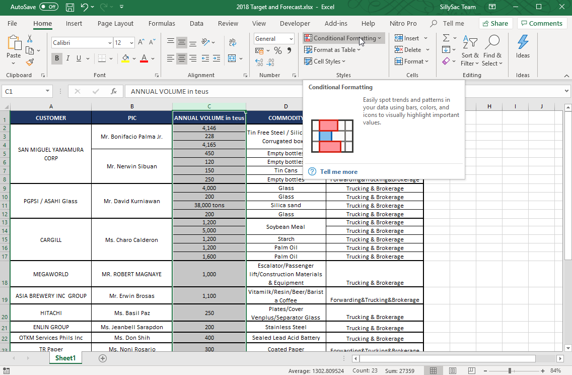
First, you have to pull up the Excel file where you have applied the conditional formatting, or the file where you intend to apply the conditional formatting to. In the example below, we have applied conditional formatting to the C column so that all values less than 1,000 will be highlighted in red.

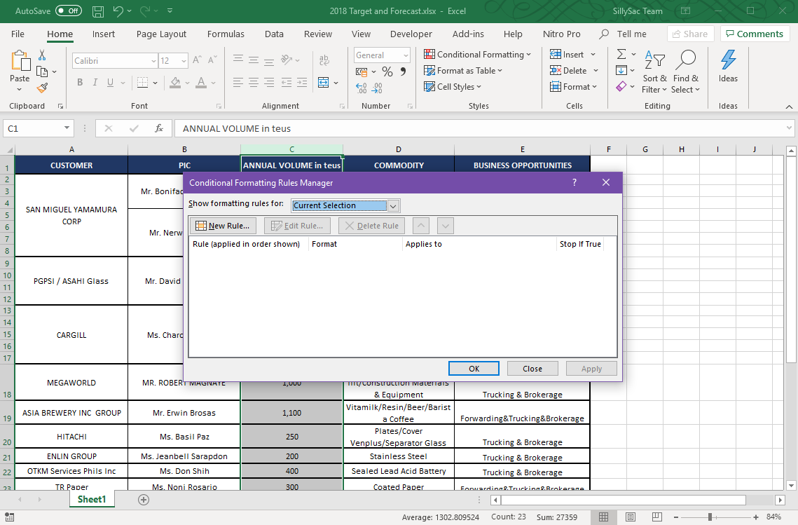
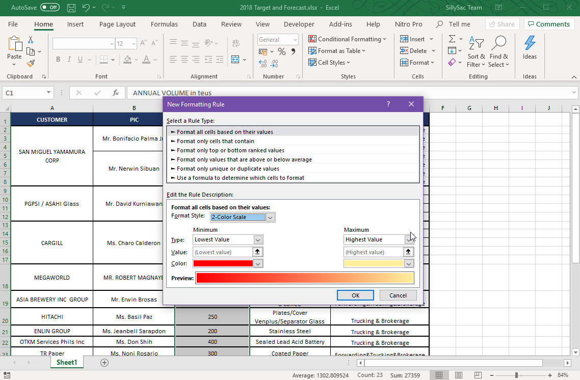
To prevent empty cells from being formatted, first you need to select the column, then go to Conditional Formatting under the Home tab in the Ribbon. Here, select Manage Rules. A new window will open, which contains New Formatting Rule. Here, you will see different rule types, which you can customize.

If you want to skip conditional formatting for blank cells, select ‘Format only cells that contain’ and select ‘Blank’ under the Edit the Rule Description. This is under the ‘Format only cells with’ that contains a drop-down list. Once you have selected ‘Blanks’ click on OK. Then, you will return to the Rule Manager window. The new rule for conditional formatting which you have added will now be listed here. Select the ‘Stop if true’ option. Then, you can add additional formatting conditions as you please. If you have other formatting conditions, make sure the one that you have created appears for blank cells at the top of the list. Then, to move it, just select the rule and use the arrow buttons to move it to the very top. Click ‘Apply’ so that all the conditional formatting rules will skip blank cells within the column you have selected.

Setup Conditional Formatting for Blank Cells to Highlight Them

Remember that there’s no condition as to when you should add the rule to skip the blank cells. You can add this rule before or after adding other rules. Just make sure that the blank cell rule appears at the very top of the list and that the ‘Stop if true’ option is selected.

By default, this rule will keep empty or blank cells free of any formatting. However, if you want blank cells to be highlighted as well, you can give it a format when you create the rule in the Conditional Formatting window. To do this, just click on the ‘Format’ button next to the ‘No Format Set’ box and then select the fill color for the cell, depending on your preference.

This setup allows you to highlight empty fields especially when you’re dealing with vast tables or a complex worksheet. You can easily spot empty cells and then, as soon as you fill these up with data, the conditional formatting you have set will be applied.