How to Create PivotTables in Excel to Calculate, Summarize and Analyze Data
One of the most powerful and most widely used features of Excel is the PivotTable. A PivotTable allows you to extract the data that you need from a large, complex, and detailed data set. Many may find themselves intimidated by pivot tables. However, once you get the hang of it, you will see how easy it is. It may also help you make better sense of large data sets for better analysis. What you may not know is, Excel PivotTables are easier to learn than you think. Let’s take a look at how to create pivot tables in Excel to calculate, summarize and analyze data.
What are PivotTables?
PivotTables allow you to extract a particular set of data from a larger, more complex data set. It also allows you to “pivot” the table. Which means you can rotate the data so that you can view it from different perspectives. It’s also important to note that you merely view your select data set. You don’t add, subtract, or modify the data. In other words, you only reorganize according to the information you need.

How to Create Pivot Tables in Excel
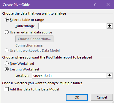
To create a pivot table, you must first enter your data into a range of rows and columns. You may also open an already existing spreadsheet with a large amount of data. Then, sort your data by a specific attribute. You must also highlight your cells to create your pivot table. The pane will appear, where you must Select a table or range under Choose the data that you want to analyze. You may also verify the cell range under the Table/Range box.
Building Your PivotTable
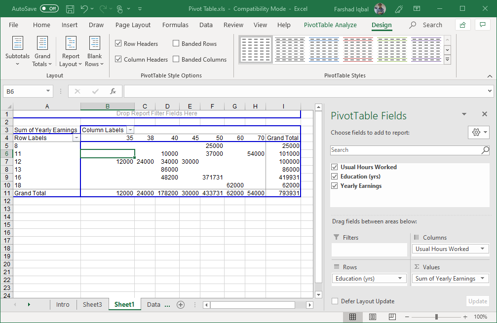
The next option is to Choose where you want the PivoTable report to be placed. Here, you may select New Worksheet. You may also choose to place it in the same worksheet where you want your PivotTable to be. Then, click OK. Now, you can start building out your Pivot table. To build out your PivotTable, you must first add a field to your PivotTable in the PivotTable Fields pane. This will auto-populate once you start to create your PivotTable. In this pane, you can customize however you want to view your data. This allows you to look at the information you have in many different ways so you can make more sense out of the information.
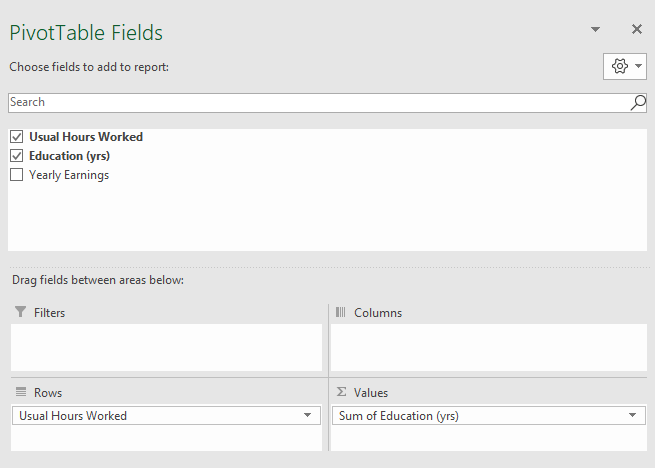
To navigate through this field pane, you can choose the fields that you want to add to your report. You may check on the check boxes the activities or reports that you want to follow. You may also drag the field to a target area of your choice, depending on how you want to organize your data. Choosing a field will help you set an identifier on which the PivotTable will be organized. Once you have your Row Labels, for example, you can then set your values by dragging a field into the Values area in the pane.
Here is a short video which shows you how to easily create a pivot table for summarizing and analyzing data.
By default, the sum of a particular field’s value is computed. Still, you have full control if you want to change your calculations into something else, like average, maximum, minimum, or other calculations.