How To Add Conditional Formatting in Google Sheets

Google has added Conditional Formatting to Google Sheets, which brings this awesome feature to online spreadsheets. Many users might be all too familiar using it with MS Excel.

Conditional Formatting feature available in Google Sheets is not only limited to differentiation of cells according to the value but also according to the date, numeral and text value. Moreover, the user is provided with the flexibility of entering any other customized differentiating value. The cell is formatted differently if any particular cell is identified by the app according to the condition applied by the user.

Adding Conditional Formatting to Spreadsheets

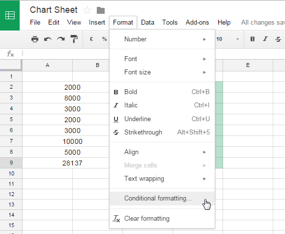
Getting Conditional Formatting on your Google Sheets is really quick and convenient. You are simply required to click on Format tab and select “Conditional Formatting” available there. The cells can be formatted based on several criteria such as:

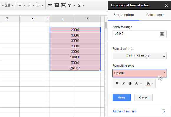
Cell is empty / cell in not empty
Date is / date if / date is after
Text contains / text does not contain / text is exactly
Custom formula
Greater than / greater than or equal to
Less than / less than or equal to
Is between / is not between
Is equal to / is no equal to

A second rule can be added after clicking Done and then you can drag & drop the rules over one another to set the order you want them to be implemented in.

You can start creating your own formatting styles or even try your hands on the ones that are available by default via the Conditional format rules box that will pop-up when you select Conditional Formatting option via the Format tab.