How to use Slicers in Excel to Filter Data

Using a Slicer in Excel is one of the best ways for you to filter your data. This is especially true if you have a large and complex data set. If you want to figure out a single category or view a specific data set under specific conditions, then a slicer can help you with that. If you want to learn how to use slicers in Excel to filter data, see the instructions given below.

What Exactly are Slicers?

Slicers are features and many Excel experts find this as their favorite feature in Excel. A slicer is actually a visual filter for your data or PivotTable or chart. A Slicer in Excel comes in the form of an interactive button. For example, if you have data on sales by categories, customers and regions, you may want to see how your sales are going in a particular product category. You may use a filter to show, in columns, the sales for a particular category. However, to make things more dynamic, you may also use a slicer on a category and just click on any region you want.

While you may use filters, you would always go back to the filter options to choose the category you want. If you want to switch to a different category, you have to go back and choose. This can take up more time especially if you have data across several categories. However, if you use a slicer in Excel, you only need to click once for every time you want to choose a category. You can easily and quickly toggle to different kinds of data.

How to Create a Slicer in Excel

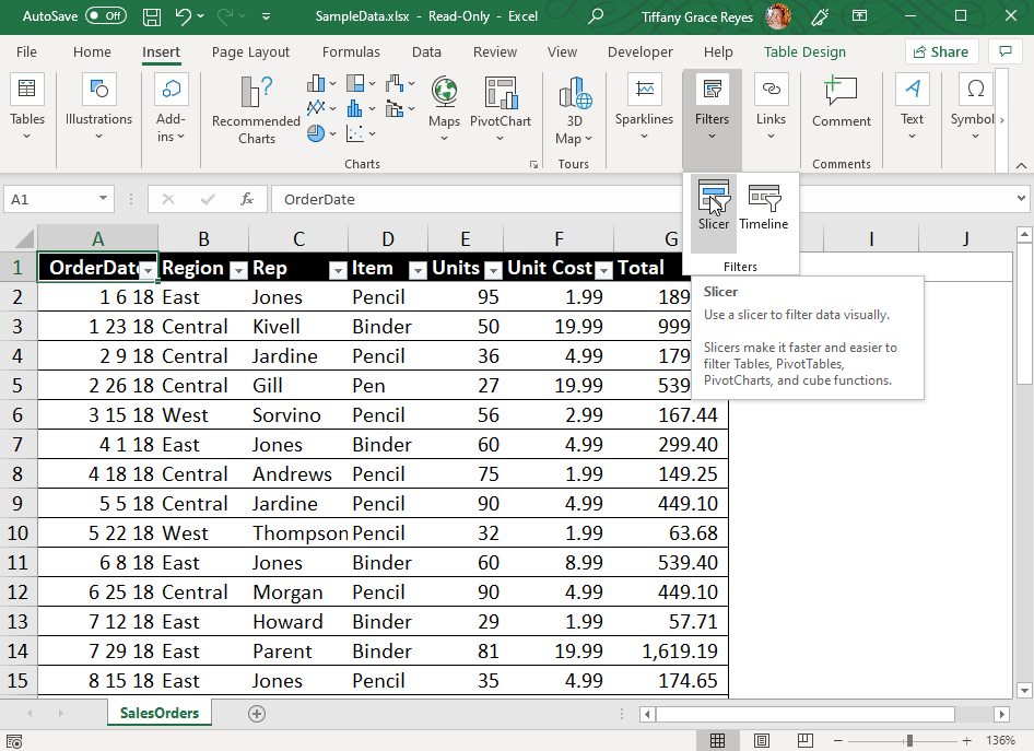
To create a slicer in Excel, you first have to make sure you are using Excel 2010 and above. Older versions do not have this function. For Excel 2010, you can only add a slicer to PivotTables. If you have Excel 2013 and later versions, you can add slicers to PivotTables and regular tables. To add slicers to regular tables, you go to the Insert tab in the ribbon, then click on the Insert Slicer button.

Now, to add slicers to PivotTables, just right-click on the PivotTable field you want and choose Add as Slicer. You may also go to the PivotTable Tools tab that activates and under Analyze, click on Insert Slicer.

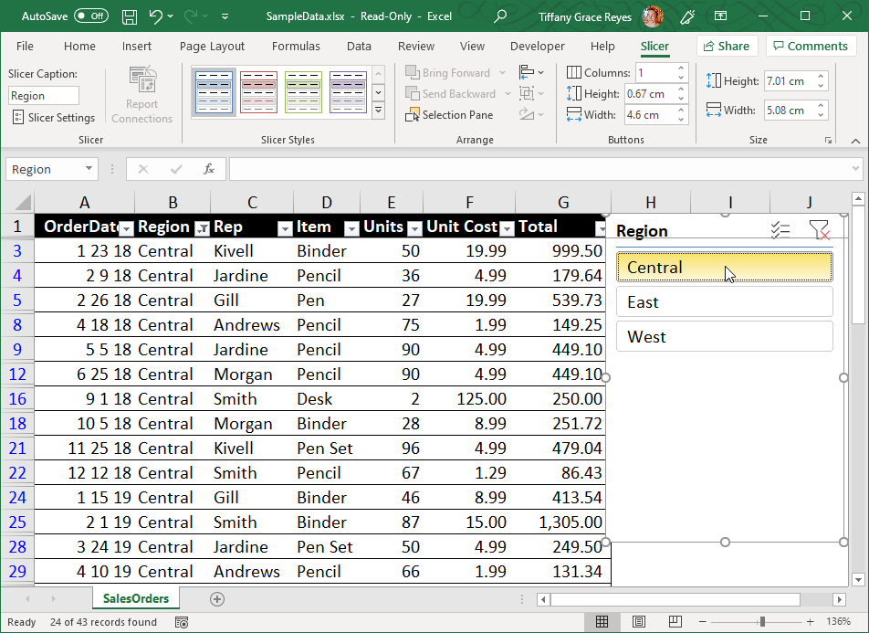
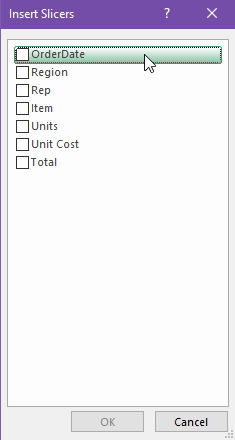
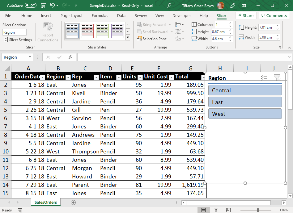
In the Insert Slicers dialog box, select the checkboxes for the fields you want to display, then click OK. You will now see a slicer created for every field that you have selected. Click on any of the slicer buttons to apply that filter to the linked regular table or PivotTable. Here is a video which shows the use of Slicers in Excel.

If you want to select more than one item, you can hold down Ctrl and then select the items that you want to show. You may also select Clean Filter to clear your choices in the slicer. You can also adjust your Slicer preferences in the Slicer tab or in the Design tab.

You can also connect a slicer to more than one PivotTable. You can do this by going to the Slicer -> Report Connections –> and then check the PivotTables you want to include or connect, then click on OK.